Chapter 4 Somwehere between basic and useful
4.1 Addressing
4.1.1 Vectors
When you deal with variables you often will want to use only a part of it in your work. Other times you will want to get rid of some values which follow certain criteria. In order to do it you need to know an ‘address’ of particular value in a vector, data frame, list etc. From now on, I will use some functions while describing it at hoc, since I believe the best way to learn them, is to use them. Lets create a vector and see what we can do with it.
addressVec <- seq(from = 1, to = 20, by = 2)
addressVec
## [1] 1 3 5 7 9 11 13 15 17 19Instead of typing all the numbers by hand, we can use seq() function, to generate it automatically. This function takes two arguments from and to, however additionally we can use option by which defines increment of the sequence. As your knowledge is growing I can tell you a secret. Often, there is no need to name all the arguments and options in functions body. In the beginning you should use the names, but the more experienced you get, you will notice that you omit them often. Actually we nearly always omit so called default options of a function. Use ?seq to check the help page for this function. You will see that it can take more options than from, to and by, but since they are predefined we don’t need to bother and type them (as long as we are OK with default settings). So, lets retype our variable definition:
addressVec <- seq(1, 20, 2)
addressVec
## [1] 1 3 5 7 9 11 13 15 17 19The results are identical. Lets get back to addressing issues. Suppose you want to check the fifth element of our addressVec variable. To do it we use variable name followed by element number in brackets (or square brackets, if you will).
addressVec[5]## [1] 9If you want to get rid of fifth element just precede it with -.
addressVec[-5]## [1] 1 3 5 7 11 13 15 17 19Easy. The thing that is worth to mention right now is that R Core Team have reason and dignity of human beings so they start numeration of elements with value 1. In some other languages, because of no sensible reasons, numeration starts with 0 – which is horribly annoying. What to do if we want to extract values of more than one element?
addressVec[1,5]## Error in addressVec[1, 5]: incorrect number of dimensionsaddressVec[-1,-5,-6]## Error in addressVec[-1, -5, -6]: incorrect number of dimensionsError occurs with warning that there is incorrect number of dimensions. That’s because vectors have only one dimension – length. Within square brackets comma separates dimensions. So when we used command [1,5] we told R to look for value that address is number 1 in first dimension and number 5 in second dimension. To correct the mistake, we need to provide a vector of numbers from first dimension. We can use c() function to create ad hoc vector inside square brackets.
addressVec[c(1,5)]## [1] 1 9addressVec[-c(1,5,6)]## [1] 3 5 7 13 15 17 19Now something more complicated. Try to figure out what code below does, and what is the result of which() function:
addressVec[which(addressVec >= 6)] <- 'o..O'
addressVec
## [1] "1" "3" "5" "o..O" "o..O" "o..O" "o..O" "o..O" "o..O" "o..O"If you have problems, you can think of this example as a composition of actions. First there is expression addressVec >=6, than we use which() function with argument from previous expression. Next the result is passed as an address. Last thing is assignment of new value to…
4.1.2 Data frames (and matrices)
When dealing with data frames, addressing is possible in two ways. First is similar to vector addressing. However, as data frames have two dimensions, you will need to express them like df[1, 2] – which tells R to look up the cell in row 1, column 2. But what if you want to check all the cells in particular row or column? Omit the number, but not the coma – like this: df[, 3]. It will display all row values from column 3. And of course you can still use vectors when addressing. This way also works for matrices.
addressDF <- data.frame(C1 = seq(1,10), C2 = seq(11,20), C3 = seq(21,30))
addressDF[5, 2]
## [1] 15addressDF[6, ]## C1 C2 C3
## 6 6 16 26addressDF[c(6, 7), 1:3]## C1 C2 C3
## 6 6 16 26
## 7 7 17 27The second option is to use $ sign followed with column name (and it works only for data frames and lists). This way, we tell R to look in whole column. If we want to display values from particular cells, we put them in brackets after column name, the same way as we do for vectors:
addressDF$C2[5]## [1] 15addressDF$C3[c(6:9)]## [1] 26 27 28 29When working with matrices you will find a lot of functions that apply to them (check help page for base package). The one you should familiarize with, if you plan on working with matrix operations are:
dim()– returns dimensions of matrixrownames()andcolnames()– to specify row and column namescbind()andrbind()– to add columns or rows to a matrix (respectively)lower.tri(),upper.tri()– lower and upper triangular part of matrixt()– matrix transpositionouter()– outer products of matrixrowsums(),rowmeans().colsums()andcolmeans()– tool to calculate sum and mean of rows or columns%*%– matrix multiplication operator (matrixOne %*% matrix2)diag()– diagonals of a matrix
You can also check help for Matrix package which contains dozens of functions to deal with matrix algebra and matrix transformations.
4.1.3 Lists
As mentioned before each list element can have different structure. Thus, addressing is kind of a mixture of all above. First you need to address element of your list. You do it with double brackets containing element number following name of variable. You can also use $ sign with name of the element. Than you use addressing the same way you address data frames, vectors or matrices.
addressList <- list(x1 = c('a', 'b'), x2 = 1:4, x3 = matrix(c(1:6), nrow = 2))
addressList[[2]]
## [1] 1 2 3 4addressList$x2[3]## [1] 3addressList[[3]]## [,1] [,2] [,3]
## [1,] 1 3 5
## [2,] 2 4 6addressList[[3]][, 3]## [1] 5 6OK, now simple task for you. There is a function called colnames() which allow us to change names in matrix variable. To use it you need to put name of matrix variable in the parentheses (like this: colnames(x)), and assign value to it (e.g. colnames(x) <- c('one', 'two')). Now change names of of columns in *matrix* that is element of list above toI`, ‘Love’, ‘R’.
4.2 Control flow
Controlling flow of function, script or whole program is the essence of programming. In general we can divide procedures in two big categories: conditional control and iteration control. In the first category we will find if...else statements. They change execution of code depending on state of input or previous results. In the second category we will find tools to repeatedly do execute some code. Typically tools to control repeating of code are for and while loops. However, in R there are special functions, which are basically for loops but have slightly better performance, and are shorter to write. We call them apply functions family.
4.2.1 if...else and ifelse statments
The simplest way to control how the code is executed are conditions. In an abstract form it is something like telling your machine: if the state is red make it blue, else make it green. The most general form it is written like below:
if (x) { #writting just X without any condtition is evaluated as x == TRUE
  function(x)
}
####rest of the code####

#Or...
if (x) {
  function(x)
} else { #in this example this block will be evaluated if x == FALSE
  function(y)
}
As you see, writing conditionals in their basic form is quite easy. If our script can be in just on of two different states while it start evaluating conditions both of above examples will be suitable. In practice it happens quite often that we need to plan different actions because of dichotomy in the results of previous actions. If our code in this place is going to make some simple things you can consider using ifelse() shortcut. It works like below:
coinToss <- sample(c(0,1), 3, replace = T)
coinToss
## [1] 1 1 1ifelse(coinToss > 0, 'Win!', 'Looser!')## [1] "Win!" "Win!" "Win!"But what if your script can have more than two states when you start evaluating conditions? You will need to use else if() structure. A simple example is below:
coinToss <- sample(c(0,1), 3, replace = T)
sumOfCoins <- sum(coinToss)# we can have four states here 0,1,2,3
sumOfCoins
## [1] 1if (sumOfCoins == 0) {
'Looser'
} else if (sumOfCoins == 1) {
'Barely alive'
} else if (sumOfCoins >= 2) {
'Big Winner!!!'
}## [1] "Barely alive"#Or because the functions realting to particular conditions are simple, you
#can make nested ifelse
ifelse(sum(sumOfCoins) == 0, 'Looser',
ifelse(sum(sumOfCoins) == 1, 'Barely alive', 'Big Winner!!!'))## [1] "Barely alive"4.2.2 for and while loops
In many cases we want to use the same function over data stored in different vectors, columns or data sets. Other time we need to make sequence of computations in which every result depends on the previous one (like, for instance, in Fibonacci sequence). In yet another situation we need to run function over data set, but only till we reach specific value. Of course, we can do everything manually, by copy-pasting code, taping ctrl+enter several times and so on. In every programming language we will find tools that help us automatize this procedures, and by side effect make them less prone to error. Those are called loops. Namely, the most common loops used are for and while. The difference between them, is that in first one we define number of iterations and in the second one we define condition that must be met so the loops is executed. In other words for (i in 1:10) {x + i} means that numbers from 1 to 10 will be added to x in a sequence. while (x < 5) {print(x <- x - 1)} on the other hand will subtract value 1 from x as long as x is greater than 0. You thing that is worth to mention is that while loops are general form and for loops are special cases. It means that it is possible to rewrite any for loop into while loop, but not the other way.
Also when working in loops you should always preallocate memory for your output. In simple words it means, that if you are writing loop, that grows the vector instead of just substitute values, R needs to copy your previous results in each iteration. Thus making a vector of length of your number of iterations (or a list) before you start a loop will save you some computational time.
To illustrate how it works in practice lets look on some simple examples:
exampleDF <- data.frame(norm = rnorm(100, 5, 1.5),
                        chisq = rchisq(100, 3),
                        pois = rpois(100, 3.33))
distroMeans <- vector('list', length(exampleDF)) #prealocate space

for (i in seq_along(exampleDF)) {
  distroMeans[[i]] <- summary(exampleDF[[i]])
}

distroMeans
## [[1]]
## Min. 1st Qu. Median Mean 3rd Qu. Max.
## 1.449 4.176 5.097 5.081 6.180 8.018
##
## [[2]]
## Min. 1st Qu. Median Mean 3rd Qu. Max.
## 0.2332 1.4592 2.3007 3.4512 4.3316 15.3055
##
## [[3]]
## Min. 1st Qu. Median Mean 3rd Qu. Max.
## 0.00 1.00 3.00 2.83 4.00 8.00Above example is very simple, and actually can be made without loop. Try to call from your console following command summary(exampleDF). This is called vectorization which will be explained few paragraphs below.
But lets get back to loops and write something that might be useful (yet very simple). Assume that you are investigating animals reproduction. You have a herd that counts 60 animals. The reproduction factor is 1.34, and survival factor is ‘0.75’. So the overall growth factor can be calculated as reproduction factor * survival factor. In each generation there is some noise in reproduction, i.e. from -3 to 2 animals are born with equal probability. This means, that number of animals in each generation directly depends of the outcome of previous generation. We want to make a chart (Fig. 4.1) to visualize population dynamics in 100 generation, thus we decide to use while (time < 101) loop.
#define initial parameters
N_0   <- 100
rf    <- 1.34
sf    <- 0.75
gf    <- rf*sf
n_gen <- 1:101
#we could repeat this inside loop, however we know the number of iterations
#thus calculating noise vector outside loop is better for performance
noise <- sample(-3:2, 100, replace = T)
t <- 1
geners <- vector('integer', length = length(n_gen))
geners[1] <- N_0
while (t < 101) {
  geners[c(t + 1)] <- floor((geners[t] * gf + noise[t]))
  t <- t + 1
}

plot(n_gen, geners, type = 'l',
     main = 'Population dynamics',
     xlab = 'generation', ylab = 'number of animals',
     col = 'blue', lty = 3)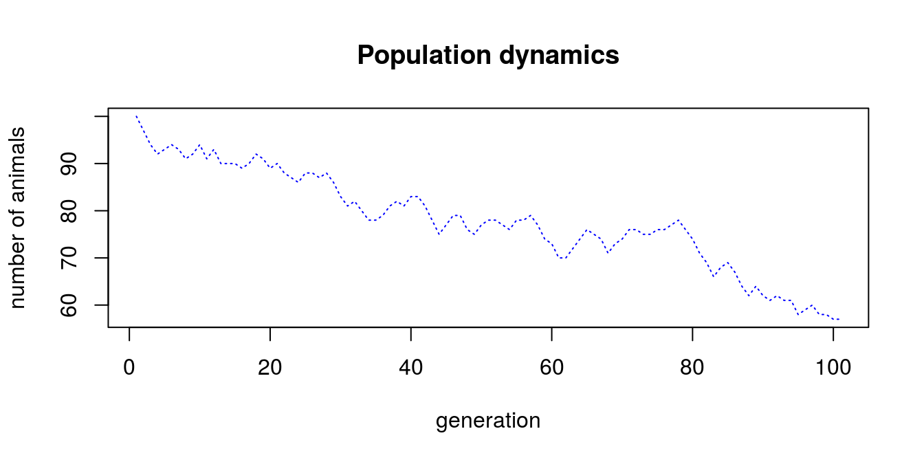
Figure 4.1: Population dynamics
It appears that we found a way to make a species extinct…
4.2.3 apply function family
For simple loops there is a shortcut. Namely, there is an apply function family that performs defined function over vector, list, matrix etc. Probably your need to use it will be reduced to lapply() and sapply() function in the beginning, thus I will focus on them here. From my experience it is better to first understand and correctly use for and while loops, than switch to lapply() and sapply() and than learn how to correctly use functions like tapply(), mapply(), vapply(). sapply() generally is the same as lapply(), the only difference is that the later function results in list of the same length as first argument. Each element of list contains results of function that was applied to the first argument. Simplified version tries to simplify results to vector, matrix or array. One tricky thing is that we we want to use function that takes more arguments than just our arguments of values over which we want to iterate we need to use a bit different syntax. In general, lets say our list is named as X, our function is SomeFunction, which takes arguments A and B (SomeFunction(A, B)). Lets asume that each element ofXis used as an argumentBin consequent iterations, whileAis fixed and equals10. The correct for of using lapply (or sapply) will be:lapply(X, SomeFunction, A = 10)`.
testApply  <- list(x = 1:10, b = rep(c(4,5), times = 5), c = rpois(5, 25))
testLapply <- lapply(testApply, mean)
testSapply <- sapply(testApply, mean)

#Here we combine previous results with another lapply,
#and use function with multiple arguments.
lapply(testSapply, rpois, n = 15)
## $x
## [1] 7 5 6 5 3 3 5 3 3 5 2 4 7 5 6
##
## $b
## [1] 2 4 5 2 3 4 3 8 6 4 8 3 3 3 5
##
## $c
## [1] 29 28 23 28 19 30 21 15 33 31 29 20 27 26 28head(sapply(testSapply, rpois, n = 15))## x b c
## [1,] 7 3 24
## [2,] 5 5 25
## [3,] 6 2 26
## [4,] 7 2 28
## [5,] 4 0 24
## [6,] 5 5 31It is also possible to use so called anonymous functions (simplifying – function that does not have name and exists temporally) as an argument.
testApplyFun <- 1:5
lapply(testApplyFun, function(x) x + 0.5)
## [[1]]
## [1] 1.5
##
## [[2]]
## [1] 2.5
##
## [[3]]
## [1] 3.5
##
## [[4]]
## [1] 4.5
##
## [[5]]
## [1] 5.5sapply(testApplyFun, function(x) x + 0.5)## [1] 1.5 2.5 3.5 4.5 5.5On the basis of previous code that calculated population dynamics, we can write general function and use it with lappy() to estimate different population dynamics depending on initial population size. Than, by addition of consequent lines representing populations with different starting points we create plot for all 4 populations (Fig. 4.2).
popDyn <- function(N_0, rf = 1.34, sf = 0.75, n_gen) {
  gf    <- rf*sf
  noise <- sample(-3:2, 100, replace = T)
  t <- 1
  geners <- vector('integer', length = n_gen)
  geners[1] <- N_0
  while (t < 101) {
  geners[c(t + 1)] <- floor((geners[t] * gf + noise[t]))
  t <- t + 1
  }
  return(geners)
}

N_0   <- c(50, 100, 150, 200, 250)
popSizes <- lapply(N_0, popDyn, n_gen = 101)

n_gen = 101
plot(1:n_gen, popSizes[[5]], type = 'l',
     main = 'Population dynamics',
     xlab = 'generation', ylab = 'number of animals',
     col = 'blue', lty = 3, ylim = c(-10, max(popSizes[[5]])))
lines(1:n_gen, popSizes[[4]], col = 'green')
lines(1:n_gen, popSizes[[3]], col = 'red')
lines(1:n_gen, popSizes[[2]], col = 'yellow')
lines(1:n_gen, popSizes[[1]], col = 'black')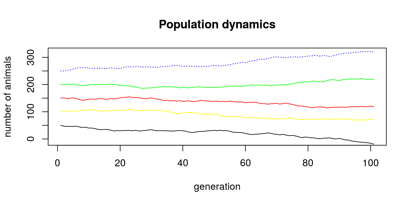
Figure 4.2: Population dynamics with different starting point
4.3 Operation on Vectors
Old proverb:
The power of R is vectorization
Indeed, vectorization is one of the most useful features of R environment. In short words, many functions are constructed in such a manner, that one can avoid using loops (since, they are often very slow). When you begin your journey with programming, you will probably not notice the difference in computation speed between vectorized way and loop way. Nonetheless, what will you find attractive, is that in many cases writing in vectorized form feels more natural. So how it works? Most basic functions are written and compiled in very fast, low level languages like C or FORTRAN. It makes computation way faster, but still we use easy R syntax. Instead of running the precompiled function on each of the elements of vector we actually can pass the vector into function – and R will know what to do. The speed is achieved because when we use function on each element, R needs to figure out what to do several (or even hundred or thousands of) times. However, when we pass whole vector into function, it needs to find out what to do only once. Sometimes, we need to use some other functions, which are not meant to process vectors (or you want to use some arbitrary functions on matrix, data frame or list). In those cases you will need to parse your data more than once to function. In R you can do it by using loops or by using so called apply family functions. When I was learning R it was most confusing thing to me, however once you get it, they become fairly easy to use. The most important difference for you as a beginner is that when using loops, you should make some memory allocation – in human language, before you run loop, you should create vector which will store results. The loops achieve highest speed when your vector can fit all the values from loop. If you do not know how big your vector will be, you need to relay on R ability to re-allocate the memory, which is S L O W. apply family hopefully takes care of this problem, so every time you know how to – use it. It will save you time and frustration of using loops. I will cover basic use of this functions later on examples.
4.4 Randomization and distribution
Random sampling is quite easy task. There is nice sample() function, that allow you to do that. You can sample from numeric, integer or even character vectors. You can even assign probabilities to particular elements of vector (we will not need that at the moment). So lets make some fun and make virtual casino. We will take two dice and will roll it 1000 times. If the sum of each result is odd and smaller than 5 we will earn 30EUR. If it is odd and higher than 5, we will get 50EUR. However if the sum is even number we loose 70EUR. Lets see if we can beat casino… First lets define our dice and rolls.
niceDice <- seq(1,6)
rollDiceOne <- sample(niceDice, 1000, replace = T)
rollDiceTwo <- sample(niceDice, 1000, replace = T)
OK, you heard about power of vectorization already, so lets sum up both vectors:
sumDiceRolls <- rollDiceOne + rollDiceTwoNext lets make some use of knowledge we got and substitute our results with some cash…
cashDiceRolls <- sumDiceRolls
cashDiceRolls[which(cashDiceRolls %% 2 == 1 & cashDiceRolls <= 5)] <- 30
cashDiceRolls[which(cashDiceRolls %% 2 == 1 & cashDiceRolls > 5)] <- 50
cashDiceRolls[which(cashDiceRolls %% 2 == 0)] <- -70
sum(cashDiceRolls)
## [1] -70000OK. What happened? We put our substitutions in very wrong order… After first two substitutions we have only even numbers in our vector… So how to fix it? Start with assigning the highest absolute value, and after all change it to negative one.
cashDiceRolls <- sumDiceRolls
cashDiceRolls[which(cashDiceRolls %% 2 == 0)] <- 70
cashDiceRolls[which(cashDiceRolls %% 2 == 1 & cashDiceRolls > 5)] <- 50
cashDiceRolls[which(cashDiceRolls %% 2 == 1 & cashDiceRolls <= 5)] <- 30
cashDiceRolls[which(cashDiceRolls  == 70)] <- -70
sum(cashDiceRolls)
## [1] -15100Now, that’s not very nice… We lost a lot of cash… But we can also track how our luck changed. Maybe we were above 0 for a while, before things got South? Or maybe we were doomed since the beginning? Lets make a plot (Fig. 4.4) to evaluate our progress.
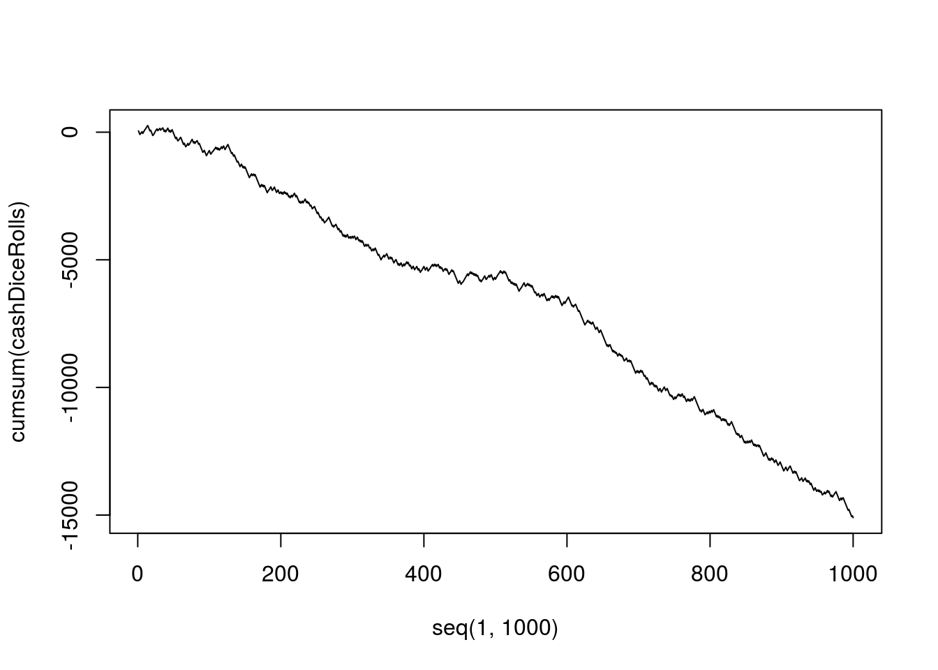
Figure 4.3: How to lose cash in casino
I think that your love to R is being deeper since I showed you how it can save a lot of your money!
In nowadays stochastic analyses are more, and more popular. With R it is quite easy to generate random numbers, sample and do all the mumbo jumbo on data. There are few functions that cover classical distributions: normal, Poisson, binomial, uniform (and few others), that are actually build in base R distribution (full list you will find here). Some more sophisticated stuff is usually covered by some packages you will need to download by yourself. You will easily find them by querying Google like this Pearson distribution in R. By using this technique it is also possible to find other useful packages for dealing with distributions (try to search for package that allows you to sample from trimmed distribution). All the distribution packages follow the same schema when naming functions. They use letters: d, p, q and r followed by abbreviation of distribution name to generate: density, distribution function, quantile function and random numbers – respectively. For instance, lets generate ten random numbers from beta distribution, with parameters 10 and 3:
rbeta(25, 10, 3)## [1] 0.7908879 0.9171753 0.7280275 0.9221093 0.7252771 0.8567831 0.8486032
## [8] 0.7670714 0.7885699 0.8840273 0.7754467 0.8560377 0.9254879 0.8793097
## [15] 0.7833065 0.9271284 0.7599927 0.8210341 0.5326531 0.8575099 0.8874445
## [22] 0.8617398 0.7338219 0.8352085 0.6764179Or we can make this nice plot (Fig. 4.4) for density of beta distribution with parameters 8 and 3:
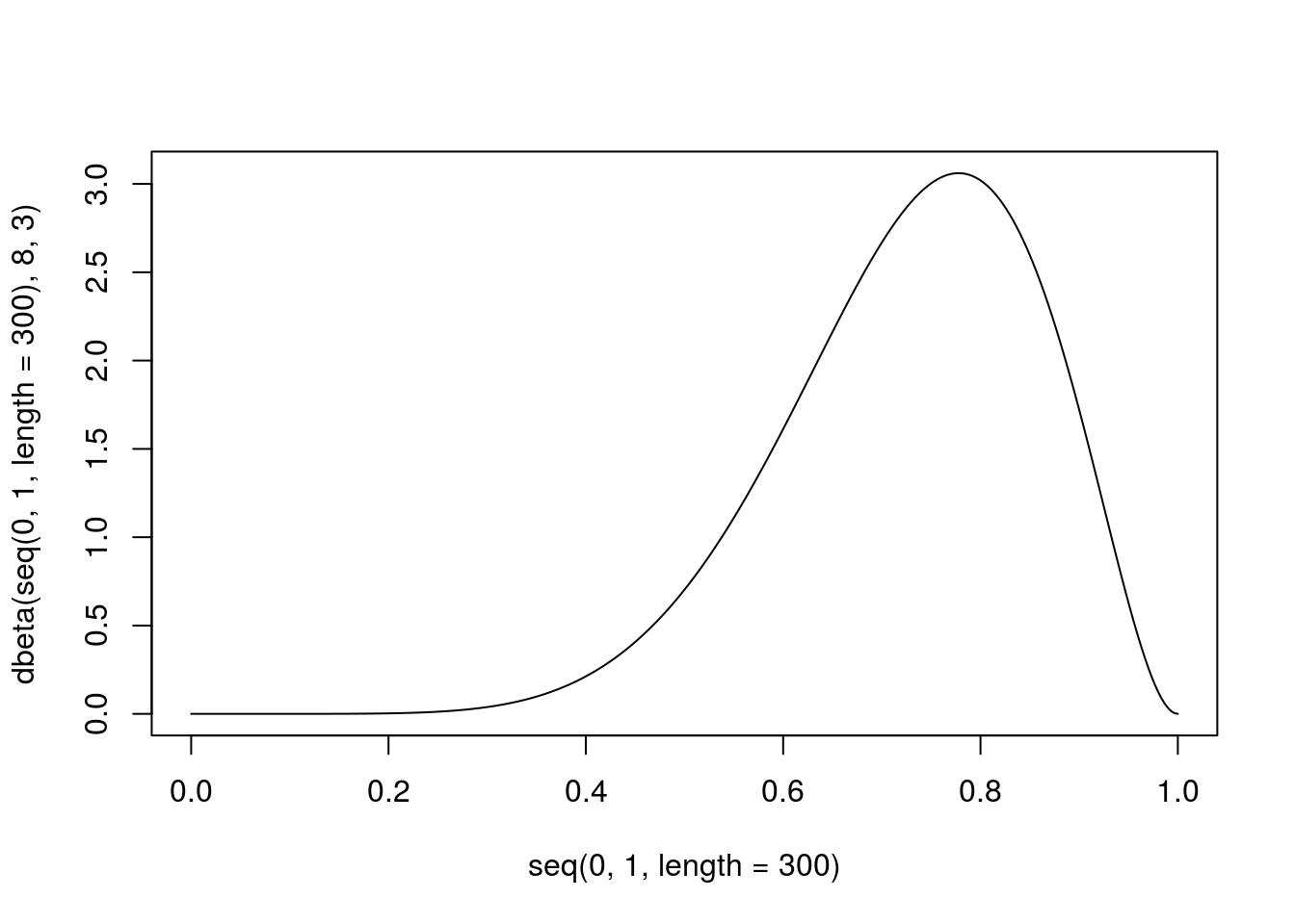
Figure 4.4: Example of beta distribution
4.5 tidyverse idea and dplyr library
The whole idea of tidy data comes from one of most famous R developers – Hadley Wickham. In on of his papers (Wickham 2014) he described procedures for generating and cleaning data in standardized manner. Many packages right now are designed to work best with data structured according to this publication. Eventually it lead to tidiverse – tools tailored for data science with common syntax and philosophy (Wickham 2017). One of the most useful packages that are included in tidiverse (Wickham 2017) are tidyr (Wickham and Henry 2018) and dplyr (Wickham et al. 2018). First helps us to swap from ‘wide’ to ‘long’ table format (and back). The second package contains set of tools to easily manipulate rows, columns or even single cells in data frame. It is extremely powerful tool, which speeds up work with data sets so much, that after few times dealing with it, you will leave traditional spread sheet forever.
4.5.1 Wide vs. long tables
Lets start with changing wide format table into long format table.
wideTable <- data.frame(male = 1:10, female = 3:12)
wideTable
## male female
## 1 1 3
## 2 2 4
## 3 3 5
## 4 4 6
## 5 5 7
## 6 6 8
## 7 7 9
## 8 8 10
## 9 9 11
## 10 10 12Than we just make a little mumbo jumbo and change it to long format:
library('tidyr')
library('dplyr')
longTable <- gather(wideTable, key = sex, value = number)
longTable[7:12, ]
## sex number
## 7 male 7
## 8 male 8
## 9 male 9
## 10 male 10
## 11 female 3
## 12 female 4That is how easy it can be done. But what if table is more complicated?
wideTable2 <- data.frame(male = 1:10,
                         female = 3:12,
                         type = rep(c('bacteria', 'virus'), times = 5),
                         group = rep(c('a', 'b'), each = 5))
wideTable2
## male female type group
## 1 1 3 bacteria a
## 2 2 4 virus a
## 3 3 5 bacteria a
## 4 4 6 virus a
## 5 5 7 bacteria a
## 6 6 8 virus b
## 7 7 9 bacteria b
## 8 8 10 virus b
## 9 9 11 bacteria b
## 10 10 12 virus bgather(wideTable2, sex, number, -c(3, 4))[7:13, ]## type group sex number
## 7 bacteria b male 7
## 8 virus b male 8
## 9 bacteria b male 9
## 10 virus b male 10
## 11 bacteria a female 3
## 12 virus a female 4
## 13 bacteria a female 5In example above, using expression -(3, 4) we indicated that we do not want to gather columns 3 and 4.
Even more complicated?
wideTable3 <- data.frame(male = rep(1:10, each = 2),
                         female = rep(3:12, times = 2),
                         type = rep(c('bacteria','virus'), times = 10),
                         group = rep(c('a','b'), each = 10),
                         day = 1:10)
wideTable3[7:13, ]
## male female type group day
## 7 4 9 bacteria a 7
## 8 4 10 virus a 8
## 9 5 11 bacteria a 9
## 10 5 12 virus a 10
## 11 6 3 bacteria b 1
## 12 6 4 virus b 2
## 13 7 5 bacteria b 3gather(wideTable3, sex, number, 1:2) %>%
spread(group, number) %>% .[7:13, ]## type day sex a b
## 7 bacteria 7 female 9 9
## 8 bacteria 7 male 4 9
## 9 bacteria 9 female 11 11
## 10 bacteria 9 male 5 10
## 11 virus 2 female 4 4
## 12 virus 2 male 1 6
## 13 virus 4 female 6 6Here our data set had additional column group storing values a and b. But imagine that group is not a variable, but it just stores the names of variables - which are a and b. This somehow might be frustrating, to decide if those are really separate variables or not. You might run into problem, that your column named environmental factor contains values: pH, conductivity, and oxygen concentration. This would be straightforward as each of this is different variable and you should spread this column into three different variables. On the other hand you might see a column that contains minimum temperature and maximum temperature. This would not be as straightforward and decision upon spreading this column would strongly depend on the context. Nonetheless, using spread() function we were able to transform values from this column as separate columns. We also used piping operator %>%. It is a shortcut, which allows us to pass the left side as an argument to the function on the right side of operator. In general it means that writing a %>% funtion(b) actually is translated into function(a, b). In the beginning this idea might be not very useful for you, but with time it will get helpful. Mainly because your code gets better structure and you can perform multiple operations without storing it in variables (which you do not want, since it consumes memory).
There is also one more common case that I should shortly mention - compound variable. It is a variable that stores multiple values in a single column. E.g. city and district, age and sex, sex and smoking, blood type and RH, etc. With tidyr is very easy to deal with it.
wideTable4 <- data.frame(type = rep(c('bacteria.a', 'virus.a'), times = 5))
wideTable4
## type
## 1 bacteria.a
## 2 virus.a
## 3 bacteria.a
## 4 virus.a
## 5 bacteria.a
## 6 virus.a
## 7 bacteria.a
## 8 virus.a
## 9 bacteria.a
## 10 virus.awideTable4 %>% separate(type, c('organism', 'type'), sep = '\\.')## organism type
## 1 bacteria a
## 2 virus a
## 3 bacteria a
## 4 virus a
## 5 bacteria a
## 6 virus a
## 7 bacteria a
## 8 virus a
## 9 bacteria a
## 10 virus a4.5.2 World of dplyr
dplyr is a library containing several useful functions, designed to ease all kinds of transformations, selections and filtering of your data frame. As the number and possibilities of functions are really huge, here I will concentrate only on some mostly used ones. Of course there is a well described documentation if you want to get deeper.
4.5.3 select columns and filter rows
Those are the most basic operations on data frames. select() function allows you to choose which columns you use. The biggest advantage of using this function instead of simple addressing, is that you can use some special functions inside it: starts_with(), ends_with(), contains(), matches(), num_range() which are helpful when using large data sets with numerous columns. There is also similar function rename() which can be used to change variable names, but in results (contrary to select()) it keeps all the variables. Lets look how the thing works on some simple examples:
head(select(wideTable3, starts_with('gr')), 3)## group
## 1 a
## 2 a
## 3 ahead(select(wideTable3, -starts_with('gr')), 3)## male female type day
## 1 1 3 bacteria 1
## 2 1 4 virus 2
## 3 2 5 bacteria 3head(select(wideTable3, contains('ale')), 3)## male female
## 1 1 3
## 2 1 4
## 3 2 5head(rename(wideTable3, Male = male), 3)## Male female type group day
## 1 1 3 bacteria a 1
## 2 1 4 virus a 2
## 3 2 5 bacteria a 3Filtering rows is also straightforward. Inside function filter() you can use logical operators (&, |, xor, !), comparisons (e.g. == or >=), or functions (is.na(), between(), near()).
filter(wideTable3, group == 'a')## male female type group day
## 1 1 3 bacteria a 1
## 2 1 4 virus a 2
## 3 2 5 bacteria a 3
## 4 2 6 virus a 4
## 5 3 7 bacteria a 5
## 6 3 8 virus a 6
## 7 4 9 bacteria a 7
## 8 4 10 virus a 8
## 9 5 11 bacteria a 9
## 10 5 12 virus a 10filter(wideTable3, type != 'bacteria')## male female type group day
## 1 1 4 virus a 2
## 2 2 6 virus a 4
## 3 3 8 virus a 6
## 4 4 10 virus a 8
## 5 5 12 virus a 10
## 6 6 4 virus b 2
## 7 7 6 virus b 4
## 8 8 8 virus b 6
## 9 9 10 virus b 8
## 10 10 12 virus b 10filter(wideTable3, near(female, 5))## male female type group day
## 1 2 5 bacteria a 3
## 2 7 5 bacteria b 34.5.4 mutate and transmute
Both functions are widely used in data manipulation in R. Their main purpose is to create new variable (usually from existing ones) in data frame. Lets look on examples:
select(wideTable3, male) %>%
  mutate(cumulativeMaleSum = cumsum(male)) %>%
  head(5)
## male cumulativeMaleSum
## 1 1 1
## 2 1 2
## 3 2 4
## 4 2 6
## 5 3 9select(wideTable3, male, female) %>%
mutate(cumulativeMaleSum = cumsum(male),
femaleLog = log(female),
cumSumFemaleLog = cumsum(femaleLog)) %>%
head(5)## male female cumulativeMaleSum femaleLog cumSumFemaleLog
## 1 1 3 1 1.098612 1.098612
## 2 1 4 2 1.386294 2.484907
## 3 2 5 4 1.609438 4.094345
## 4 2 6 6 1.791759 5.886104
## 5 3 7 9 1.945910 7.832014As you can see in second example, when we use mutate() function, the newly created variables (in this example femaleLog) are available immediately so we can use them to create another variable (in this case cumSumFemaleLog) within one function call. In this example, I also used piping operator, because calculating intermediate steps and storing them as a result, which can be used later is useless, as we are interested only in the final outcome. The biggest advantage of this procedure is that we keep our Environment clean and preserve memory – which is very important in long and memory consuming projects. Last but not least, the difference between mutate() and transmute() is that the latter do not preserve all variables, only the ones you created.
4.5.5 group_by and summarise
summarise() is commonly used function on grouped data. It allows to calculate many typical descriptive statistics (like mean() or quantile()) for particular groups in you data set, as well as it can count number of observations (n() function), or number of unique observations (distinct()). To see how it works in practice lets look back on our example and calculate mean value for males and female, as well as day range and number of cases for groups derived from type.
wideTable3 %>%
  group_by(type) %>%
  summarise(meanF = mean(female),
            meanM = mean(male),
            numberOfDays = (range(day)[2]-range(day)[1]),
            numberOfCases = n())
## # A tibble: 2 x 5
## type meanF meanM numberOfDays numberOfCases
## <fct> <dbl> <dbl> <int> <int>
## 1 bacteria 7 5.5 8 10
## 2 virus 8 5.5 8 10Easy.
4.6 Is there anything more in dplyr library?
Yes. Actually I presented here only very very tiny fracture of dplyr possibilities just to familiarize you with syntax and using piping operator. When you go deeper into world of data frames transformation, you will find other commonly used functions like: different kinds of joining data frames (similar to SQL joining tables), conditional selecting, filtering, renaming rows and columns, extracting values or arranging your data frame. Thankfully this procedures are so common that even if you won’t grasp it immediately from functions description, you will still find hundreds of tutorials on the web, or help in StackOverflow.
References
Wickham, Hadley. 2014. “Tidy Data.” Journal of Statistical Software 59 (10): 1–23.
Wickham, Hadley. 2017. Tidyverse: Easily Install and Load the ’Tidyverse’. https://CRAN.R-project.org/package=tidyverse.
Wickham, Hadley, and Lionel Henry. 2018. Tidyr: Easily Tidy Data with ’Spread()’ and ’Gather()’ Functions. https://CRAN.R-project.org/package=tidyr.
Wickham, Hadley, Romain François, Lionel Henry, and Kirill Müller. 2018. Dplyr: A Grammar of Data Manipulation. https://CRAN.R-project.org/package=dplyr.