Chapter 2 Introduction
2.1 Audience
I wrote this small book for all those who are new to programming, as well for those who are new to R language. I tried to cover all the necessary knowledge you need to be familiarize with to start basic work in R in a compact way. I also tried to avoid things that may overwhelm or confuse people who are new to programming (like code efficiency). However if you want to play more, with more complex coding you need to read a lot from other sources. You will find some advises what should you do next in last chapter (9) of this book.
2.2 What this book is not about?
Mainly this book not on any advanced R. I do not cover here things like function factories, creating packages or S3 classes. It also do not cover specific R application in detail, like statistics, predictive modeling or text analyses. Finally this book will not cover programming paradigms such as Test Driven Development or Meta-programming. There are plenty of well written resources that go really deep in those applications.
2.3 RStudio
Before we jump into coding, you should first get familiar with RStudio (RStudio Team 2016). It is so called Integrated Development Environment (IDE), which has built-in functionalities to make work easier. This IDE is typically used with 4 different windows:
- Source - where you can write scripts;
- Console - where scripts are executed;
- ‘Environmental’ - it’s adjustable window, usually containing Environemnt, History and Version Control panes;
- ‘Files’ - also adjustable, usually you will find here File, Packages, Help and Plots panes.
2.4 Few tips to make life easier
From menu choose Tools > Global options. Now choose Code and Editing pane, tick box Insert spaces for Tab and assure that Tab width is set to 2. Next, in Display pane, check following tick-boxes: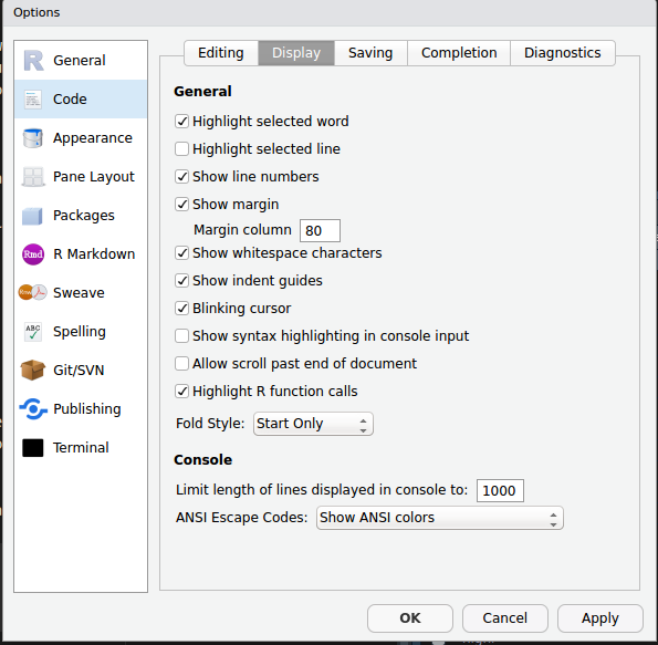
Figure 2.1: Code display options
- Highlight selected word
- Show line number
- Show margin (and set margin column to 80)
- Show whitespace characters
- Highlite R function calls
Generally speaking those options, do not influence how your code is performed, but will allow you to write cleaner and read easier. You can also change colors of your environment in Appearance.
2.5 Installing packages
In your ‘Files’ window, you will find Packages pane, which contains Install button. You can use it now, to install packages needed to perform exercises from this book. The packages are: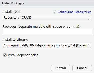
Figure 2.2: Installation window
- deSolve (Soetaert, Petzoldt, and Setzer 2018)
- fitdistrplus (Delignette-Muller, Dutang, and Siberchicot 2017)
- mc2d (Pouillot 2017)
- minpack.lm (Elzhov et al. 2016)
- nls2 (Grothendieck 2013)
- nlsMicrobio (Baty and Delignette-Muller 2014)
- segmented (Muggeo 2017)
- tidyverse (Wickham 2017; Wickham et al. 2018; Wickham and Chang 2016; Wickham and Henry 2018)
- viridis (Garnier 2018)
Now every time you need functions from specific package in library you can just tick box next to package name, and RStudio will load it for you.
2.6 Conventions
In this book, we will use following conventions:
- Names of programs and packages are in Bold.
- All other names e.g. names of panes menu items as well as things that needs to be stressed are in italics.
- Function names and variables are always written in inline code e.g.
t.test()orx. - File names are written in inline code e.g.
foo.txt. - Citations are in APA style, and ‘clickable’ e.g.click on the name and year of knitr package citation (Xie 2015).
- Code chunks are in blocks and result lines start with ##
rnorm(10, 1, 0.5)## [1] 0.74776654 0.65335854 1.86435057 0.47452808 0.06063708 1.21071321
## [7] 1.03416903 0.69726630 1.04683980 0.54020081- There are no
>(prompt) signs in code chunks. - Figures are floating - meaning, that they are not always immediately after they are mentioned in text.
- Tables are in longtable format (meaning they are not floating and might be multipage) e.g.
knitr::kable(
  head(iris, 25), caption = 'Example table',
  booktabs = TRUE, longtable = TRUE
)| Sepal.Length | Sepal.Width | Petal.Length | Petal.Width | Species |
|---|---|---|---|---|
| 5.1 | 3.5 | 1.4 | 0.2 | setosa |
| 4.9 | 3.0 | 1.4 | 0.2 | setosa |
| 4.7 | 3.2 | 1.3 | 0.2 | setosa |
| 4.6 | 3.1 | 1.5 | 0.2 | setosa |
| 5.0 | 3.6 | 1.4 | 0.2 | setosa |
| 5.4 | 3.9 | 1.7 | 0.4 | setosa |
| 4.6 | 3.4 | 1.4 | 0.3 | setosa |
| 5.0 | 3.4 | 1.5 | 0.2 | setosa |
| 4.4 | 2.9 | 1.4 | 0.2 | setosa |
| 4.9 | 3.1 | 1.5 | 0.1 | setosa |
| 5.4 | 3.7 | 1.5 | 0.2 | setosa |
| 4.8 | 3.4 | 1.6 | 0.2 | setosa |
| 4.8 | 3.0 | 1.4 | 0.1 | setosa |
| 4.3 | 3.0 | 1.1 | 0.1 | setosa |
| 5.8 | 4.0 | 1.2 | 0.2 | setosa |
| 5.7 | 4.4 | 1.5 | 0.4 | setosa |
| 5.4 | 3.9 | 1.3 | 0.4 | setosa |
| 5.1 | 3.5 | 1.4 | 0.3 | setosa |
| 5.7 | 3.8 | 1.7 | 0.3 | setosa |
| 5.1 | 3.8 | 1.5 | 0.3 | setosa |
| 5.4 | 3.4 | 1.7 | 0.2 | setosa |
| 5.1 | 3.7 | 1.5 | 0.4 | setosa |
| 4.6 | 3.6 | 1.0 | 0.2 | setosa |
| 5.1 | 3.3 | 1.7 | 0.5 | setosa |
| 4.8 | 3.4 | 1.9 | 0.2 | setosa |
References
RStudio Team. 2016. RStudio: Integrated Development Environment for R. Boston, MA: RStudio, Inc. http://www.rstudio.com/.
Soetaert, Karline, Thomas Petzoldt, and R. Woodrow Setzer. 2018. DeSolve: Solvers for Initial Value Problems of Differential Equations (’Ode’, ’Dae’, ’Dde’). https://CRAN.R-project.org/package=deSolve.
Delignette-Muller, Marie-Laure, Christophe Dutang, and Aurélie Siberchicot. 2017. Fitdistrplus: Help to Fit of a Parametric Distribution to Non-Censored or Censored Data. https://CRAN.R-project.org/package=fitdistrplus.
Pouillot, Regis. 2017. Mc2d: Tools for Two-Dimensional Monte-Carlo Simulations. https://CRAN.R-project.org/package=mc2d.
Elzhov, Timur V., Katharine M. Mullen, Andrej-Nikolai Spiess, and Ben Bolker. 2016. Minpack.lm: R Interface to the Levenberg-Marquardt Nonlinear Least-Squares Algorithm Found in Minpack, Plus Support for Bounds. https://CRAN.R-project.org/package=minpack.lm.
Grothendieck, G. 2013. Nls2: Non-Linear Regression with Brute Force. https://CRAN.R-project.org/package=nls2.
Baty, Florent, and Marie-Laure Delignette-Muller. 2014. NlsMicrobio: Nonlinear Regression in Predictive Microbiology. https://CRAN.R-project.org/package=nlsMicrobio.
Muggeo, Vito M. R. 2017. Segmented: Regression Models with Break-Points / Change-Points Estimation. https://CRAN.R-project.org/package=segmented.
Wickham, Hadley. 2017. Tidyverse: Easily Install and Load the ’Tidyverse’. https://CRAN.R-project.org/package=tidyverse.
Wickham, Hadley, Romain François, Lionel Henry, and Kirill Müller. 2018. Dplyr: A Grammar of Data Manipulation. https://CRAN.R-project.org/package=dplyr.
Wickham, Hadley, and Winston Chang. 2016. Ggplot2: Create Elegant Data Visualisations Using the Grammar of Graphics. https://CRAN.R-project.org/package=ggplot2.
Wickham, Hadley, and Lionel Henry. 2018. Tidyr: Easily Tidy Data with ’Spread()’ and ’Gather()’ Functions. https://CRAN.R-project.org/package=tidyr.
Garnier, Simon. 2018. Viridis: Default Color Maps from ’Matplotlib’. https://CRAN.R-project.org/package=viridis.
Xie, Yihui. 2015. Dynamic Documents with R and Knitr. 2nd ed. Boca Raton, Florida: Chapman; Hall/CRC. http://yihui.name/knitr/.