Chapter 8 Simple workflow
8.1 Data
We manage to go through whole introduction to R’s Galaxy. But that’s not the end. For a final word I would like to go with you with once again through some of the stuff you will need more or less in your everyday job. We will use R to see, how we can predict some values in basic microbiology.
First we need a data set. I downloaded data from deposited in ComBase for Bacillus cereus in broth with conditions as follows: pH = 6.1, water activity (aw) = 0.974, sodium chloride in environment = 4.5%, temperatures = 15, 16, 20, 22, 30 degrees Celsius. This data comes from Food Standards Agency, UK, and is hardcoded (so you can copy-paste) in the end of this chapter.
8.2 Exploaratory visualisation and setup
We will start with visually inspecting this data set.
ggplot(BcDF, aes(x = Time, y = LogC)) +
  geom_point(aes(colour = resID)) +
  facet_wrap(~Temp)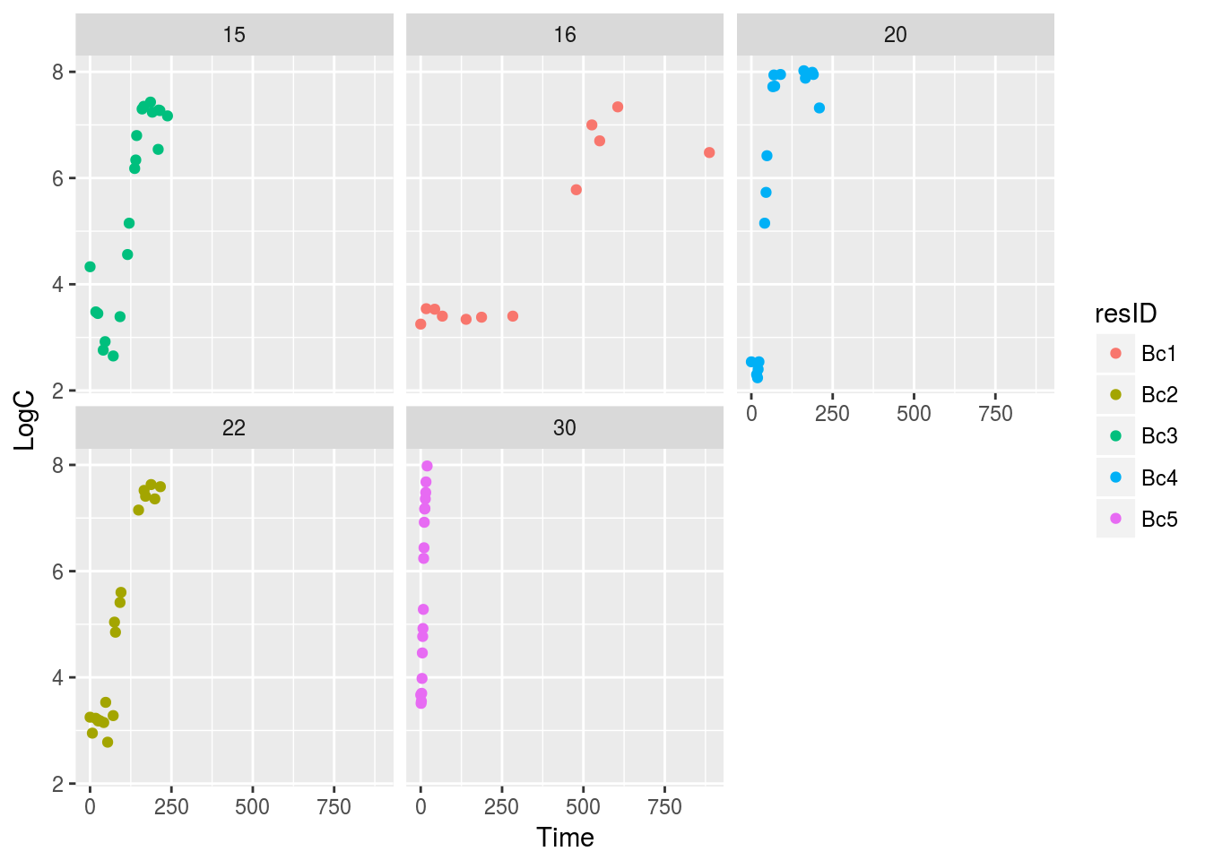
Figure 8.1: Growths in temperature range
Unfortunately, one plot on Fig. 8.1 (30 degrees Celsius) is bit compressed, so lets isolate it and look closer on the points (Fig. 8.2).
BcDFsub39 <- subset(BcDF, Temp == 30)
ggplot(BcDFsub39, aes(x = Time, y = LogC)) +
  geom_point()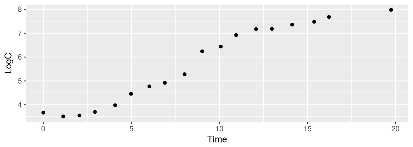
Figure 8.2: Growth in 30 deg. C
It seems that there is at least short lag phase in each of the growth temperatures. We will use nlsMicrobio package, which contains some models, that we will use to estimate \(\mu_{max}\). First we will split, whole data frame into list of data frames – one for each temperature. Than we will use our good friend lapply() to change names of columns in all data sets so it fits needs of our function.
BcList <- split(BcDF, f= BcDF$resID)
BcList <- lapply(BcList, setNames, nm = c('t',  'LOG10N', 'Temp', 'resID'))
From plots above (i.e., Fig. 8.1 and Fig. 8.2) we make an assumption that all of those growth curves have shorter or longer lag phase.
8.3 Growth models
It would be nice to use trilinear (Buchanan) and Baranyi model to estimate \(\mu_{max}\). However writing it by hand is error prone, we can use predefined models from nlsMicrobio package (and that is why we need precise names of columns). Lets see how models look:
baranyi## LOG10N ~ LOG10Nmax + log10((-1 + exp(mumax * lag) + exp(mumax *
## t))/(exp(mumax * t) - 1 + exp(mumax * lag) * 10^(LOG10Nmax -
## LOG10N0)))
## <environment: namespace:nlsMicrobio>buchanan## LOG10N ~ LOG10N0 + (t >= lag) * (t <= (lag + (LOG10Nmax - LOG10N0) *
## log(10)/mumax)) * mumax * (t - lag)/log(10) + (t >= lag) *
## (t > (lag + (LOG10Nmax - LOG10N0) * log(10)/mumax)) * (LOG10Nmax -
## LOG10N0)
## <environment: namespace:nlsMicrobio>To estimate trilinear model we could also use segmented package, however than we would use different approach to solve the problem – we would estimate breakpoints or knots and than fit linear regression for each segment. The problem with this approach is that because of data in lag and stationary phase, with this method we would obtain slope values \(\neq 0\) for those phases.
Unfortunately, when using non-linear regression algorithms we sometimes run into trouble and cannot really estimate values we are interested in. Sometimes we need to make small changes in initial values that we parse as function arguments. In other times, R is unable to make estimations due to data structure. The main problem is that there is no one size fits all solution, and often finding best way to solve a problem is an iterative process of manually finding best starting parameters or using multiple functions to find the working one. Below we attempt to find \(\mu_{max}\) with Baranyi and Buchanan approach.
bar1.nls <- nls(baranyi, BcList$Bc1,
                list(lag = 200, mumax = 0.03, LOG10N0 = 3, LOG10Nmax = 6.5),
                control = nls.control(maxiter = 500))
## Error in nls(baranyi, BcList$Bc1, list(lag = 200, mumax = 0.03, LOG10N0 = 3, : step factor 0.000488281 reduced below 'minFactor' of 0.000976562bar2.nls <- nls(baranyi, BcList$Bc2,
list(lag = 2, mumax = 0.5, LOG10N0 = 2, LOG10Nmax = 8))## Warning in numericDeriv(form[[3L]], names(ind), env): NaNs produced## Error in numericDeriv(form[[3L]], names(ind), env): Missing value or an infinity produced when evaluating the modelbar3.nls <- nls(baranyi, BcList$Bc3,
list(lag = 5, mumax = 0.01, LOG10N0 = 3, LOG10Nmax = 6))## Error in numericDeriv(form[[3L]], names(ind), env): Missing value or an infinity produced when evaluating the modelbar4.nls <- nls(baranyi, BcList$Bc4,
list(lag = 1, mumax = 0.5, LOG10N0 = 2, LOG10Nmax = 8))
bar5.nls <- nls(baranyi, BcList$Bc5,
list(lag = 1, mumax = 0.5, LOG10N0 = 3, LOG10Nmax = 8))OK. That is a bit worrying. We were able to solve equations only for two data sets. One solution we can try is to use minipack.lm which uses different approach which often works better than standard nls function. We will also allow more iterations of algorithm, which is second common solution.
bar1.nlsLM <- nlsLM(baranyi, BcList$Bc1,
                    list(lag = 200, mumax = 0.03, LOG10N0 = 3, LOG10Nmax = 6.5),
                    control = nls.lm.control(maxiter = 500))
summary(bar1.nlsLM)
##
## Formula: LOG10N ~ LOG10Nmax + log10((-1 + exp(mumax * lag) + exp(mumax *
## t))/(exp(mumax * t) - 1 + exp(mumax * lag) * 10^(LOG10Nmax -
## LOG10N0)))
##
## Parameters:
## Estimate Std. Error t value Pr(>|t|)
## lag 4.622e+02 1.121e+06 0.00 1
## mumax 3.515e-01 2.497e+04 0.00 1
## LOG10N0 3.406e+00 9.269e-02 36.74 3.30e-10 ***
## LOG10Nmax 6.880e+00 1.416e-01 48.59 3.56e-11 ***
## ---
## Signif. codes: 0 '***' 0.001 '**' 0.01 '*' 0.05 '.' 0.1 ' ' 1
##
## Residual standard error: 0.2452 on 8 degrees of freedom
##
## Number of iterations to convergence: 41
## Achieved convergence tolerance: 1.49e-08BaranyiBc1 <- summary(bar1.nlsLM)$parametersLets substitute variables in equation (later I’ll show you haw to do it automatically):
LOG10N ~ LOG10Nmax + log10((-1 + exp(mumax * lag) + exp(mumax * t))/(exp(mumax * t) - 1 + exp(mumax * lag) * 10^(LOG10Nmax - LOG10N0
with calculated ones and see how predicted curve fits our data (Fig. 8.3).
xBarBc1 <- 1:800
predBarBc1 <- 6.880 +
  log10((-1 + exp(0.3537 * 462.2242) +
           exp(0.3515 * xBarBc1))/
          (exp(0.3515 * xBarBc1) - 1 +
exp(0.3515 * 462.2242) * 10^(6.880 - 3.406)))plot(BcList$Bc1$t, BcList$Bc1$LOG10N)
lines(predBarBc1~xBarBc1)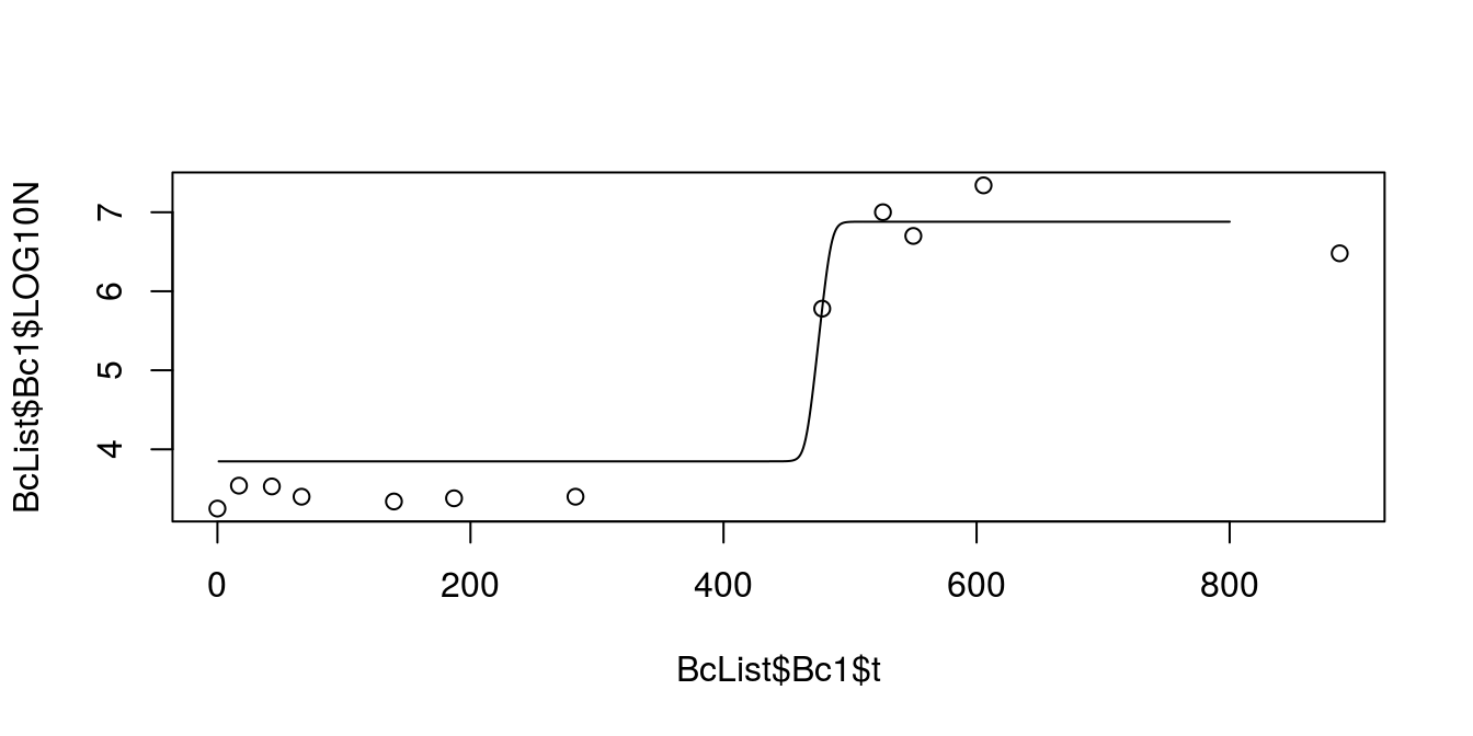
Figure 8.3: Predicted growth from Baranyi equation for Bc1 dataset
This does not look like a good fit. Yet another solution to this problem is to use package segmented. It’s not the most elegant solution to the problem, but hey, our data is not the best one as well.
segmented1.lm <- lm(LOG10N~1, data = BcList$Bc1) %>%
  segmented(seg.Z = ~t,
            psi = c(200, 400),
            control = seg.control(it.max = 500, n.boot = 300))
Segmented1 <- list(confint.segmented(segmented1.lm),slope(segmented1.lm))
** NOTE: You should rather use formula: lm(LOG10N~t, data = BcList$Bc1), however for unknown reasons when using
bookdownbuild functions fails to calculate linear model. So, till I find a solution to this problem we’ll stick to simplified one.
Now we make some quick plot (Fig. 8.4) to check how does the prediction fits data.
plot(segmented1.lm)
points(BcList$Bc1$LOG10N~BcList$Bc1$t)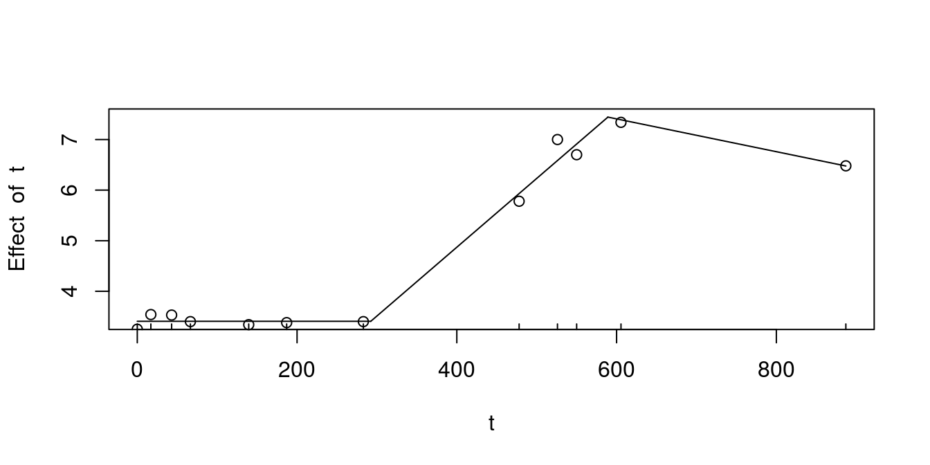
Figure 8.4: Predicted growth from segmented regression for Bc1 dataset
As I stated before, the lag and stationary phase segments are not nice, however slope of the growth phase seems to fit slightly better than the one calculated with nlsML() and baranyi. Also we need to remember that the more data points exist in set, and the better they are spread among independent variable range, the easier it gets to make statistical procedures, and the results will be more robust.
We can also try to fit non linear regression for buchanan with nlsML() and nls2 (the latter with brute force). Unfortunately, nls methods are quite sensitive on data and initial values, thus sometimes it takes a while to find something that makes sens or does not throw error now as singular gradient matrix at initial parameter estimates.
## Levenberg-Marquardt algorithm
buch1.nlsLM <- nlsLM(buchanan, BcList$Bc1,
                     list(lag = 200, mumax = 0.03,
                          LOG10N0 = 3, LOG10Nmax = 6.5),
                     control = nls.lm.control(maxiter = 500))
## Gauss-Newton algorithm with brute-force
buch1.nlsBF <- nls2(buchanan, data = BcList$Bc1,
                    start = list(lag = 280, mumax = 0.03,
                                 LOG10N0 = 3.5, LOG10Nmax = 7),
                    control = nls.control(maxiter = 1000,
                                          tol = 1e-01, minFactor = 1/100),
                    algorithm = 'brute-force')
BuchananBFBc1<- summary(buch1.nlsLM)$parameters
BuchananBc1<- summary(buch1.nlsBF)$parameters
And quick plot (Fig. 8.5) for visual inspection:
par(mfrow = c(1,2))
plot(BcList$Bc1$t, BcList$Bc1$LOG10N)
lines(predict(buch1.nlsLM)~BcList$Bc1$t)

plot(BcList$Bc1$t, BcList$Bc1$LOG10N)
lines(predict(buch1.nlsBF)~BcList$Bc1$t)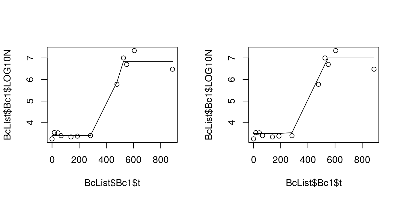
Figure 8.5: Comparission of fiting Buchanan equation with Levenberg-Marquardt and brute-force Gauss-Newton
par(mfrow = c(1,1))Lets compare our parameters estimates:
Segmented1## [[1]]
## [[1]]$t
## Est. CI(95%).l CI(95%).u
## psi1.t 292.257 132.161 452.354
## psi2.t 589.121 535.548 642.694
##
##
## [[2]]
## [[2]]$t
## Est. St.Err. t value CI(95%).l CI(95%).u
## slope1 0.0000000 NA NA NA NA
## slope2 0.0136000 0.0040287 3.3758 0.0040738 0.02312700
## slope3 -0.0032442 0.0010493 -3.0916 -0.0057254 -0.00076286BaranyiBc1## Estimate Std. Error t value Pr(>|t|)
## lag 462.2241887 1.120639e+06 4.124648e-04 9.996810e-01
## mumax 0.3515197 2.497031e+04 1.407751e-05 9.999891e-01
## LOG10N0 3.4057143 9.269492e-02 3.674111e+01 3.301879e-10
## LOG10Nmax 6.8800000 1.415938e-01 4.858969e+01 3.561034e-11BuchananBc1## Estimate Std. Error t value Pr(>|t|)
## lag 280.00 26.043862981 10.751093 4.930689e-06
## mumax 0.03 0.003968372 7.559775 6.547676e-05
## LOG10N0 3.50 0.128057657 27.331439 3.461481e-09
## LOG10Nmax 7.00 0.181100875 38.652491 2.205201e-10BuchananBFBc1## Estimate Std. Error t value Pr(>|t|)
## lag 354.25006466 55.09540195 6.429757 2.026158e-04
## mumax 0.04610793 0.01690905 2.726819 2.597327e-02
## LOG10N0 3.40424344 0.09420648 36.135981 3.768335e-10
## LOG10Nmax 6.84343632 0.14390277 47.555974 4.227236e-11As you can see, all the methods differ in their estimates (for Baranyi it \(\mu_{max}\) is expressed as natural logarithm, so we can use equation \(log_{10}(x) = \frac{ln(x)}{ln(10)}\) to obtain value 0.1526631). Some of them work better some work worse. Sometimes they produce false convergence, sometimes they highly rely even on small changes in initial values and sometimes they just do not work with our data set. Other thing one should consider is very wise proverb:
Garbage in, garbage out.
Meaning, that even with best methods, our data set might just not be sufficient to produce reliable output. Unfortunately in many cases we need to deal somehow with this kind of data. And we should always check if our output makes sense.
But lets try to find a solution to other Bc2 and Bc3 data sets. We’ll simplify things and start estimation of parameters with Buchanan and Baranyi models using nlsLM
buch2.nlsLM <- nlsLM(buchanan, BcList$Bc2,
                    list(lag = 100, mumax = 0.03, LOG10N0 = 3, LOG10Nmax = 6.5),
                    control = nls.lm.control(maxiter = 500))
buch3.nlsLM <- nlsLM(buchanan, BcList$Bc3,
                    list(lag = 100, mumax = 0.03, LOG10N0 = 3, LOG10Nmax = 6.5),
                    control = nls.lm.control(maxiter = 500))
bar2.nlsLM <- nlsLM(baranyi, BcList$Bc2,
                list(lag = 10, mumax = 0.2, LOG10N0 = 3, LOG10Nmax = 6.5),
                control = nls.lm.control(maxiter = 500))
bar3.nlsLM <- nlsLM(baranyi, BcList$Bc3,
                list(lag = 10, mumax = 0.03, LOG10N0 = 3, LOG10Nmax = 6.5),
                control = nls.lm.control(maxiter = 500))
Hurray! No errors… for now at least. Now, we can use our variable that contains estimated parameters to make prediction. We will need new data frame containing values for which we want to make prediction. Because, we want also to plot predicted lines (to check how they fit to our data sets), we can predict values along sequence of numbers from 1 to 270. So, lets inspect visually how our models fit to data (Fig. 8.6).
newTime <- data.frame(t = 1:270)
predBuch2 <- predict(buch2.nlsLM, newdata = newTime)
predBuch3 <- predict(buch3.nlsLM, newdata = newTime)
predBar2 <- predict(bar2.nlsLM, newdata = newTime)
predBar3 <- predict(bar3.nlsLM, newdata = newTime)

#4 plots in one picture 2 x 2
par(mfrow = c(2,2))
plot(predBuch2 ~ newTime$t, type = 'l', col = 'red',
     main = 'Buchanan', sub = 'dataset Bc2', cex.main = 0.75, cex.sub = 0.6,
     xlab = 'time', ylab = 'Log10N', cex.lab = 0.6)
  points(BcList$Bc2$t, BcList$Bc2$LOG10N,
         col = 'blue', pch = 15)

plot(predBuch3 ~ newTime$t, type = 'l', col = 'red',
     main = 'Buchanan', sub = 'dataset Bc3', cex.main = 0.75, cex.sub = 0.6,
     xlab = 'time', ylab = 'Log10N', cex.lab = 0.6)
  points(BcList$Bc3$t, BcList$Bc3$LOG10N,
         col = 'blue', pch = 15)

plot(predBar2 ~ newTime$t, type = 'l', col = 'red',
     main = 'Baranyi', sub = 'dataset Bc2', cex.main = 0.75, cex.sub = 0.6,
     xlab = 'time', ylab = 'Log10N', cex.lab = 0.6)
  points(BcList$Bc2$t, BcList$Bc2$LOG10N,
         col = 'blue', pch = 15)

plot(predBar3 ~ newTime$t, type = 'l', col = 'red',
     main = 'Baranyi', sub = 'dataset Bc3', cex.main = 0.75, cex.sub = 0.6,
     xlab = 'time', ylab = 'Log10N', cex.lab = 0.6)
  points(BcList$Bc3$t, BcList$Bc3$LOG10N,
         col = 'blue', pch = 15)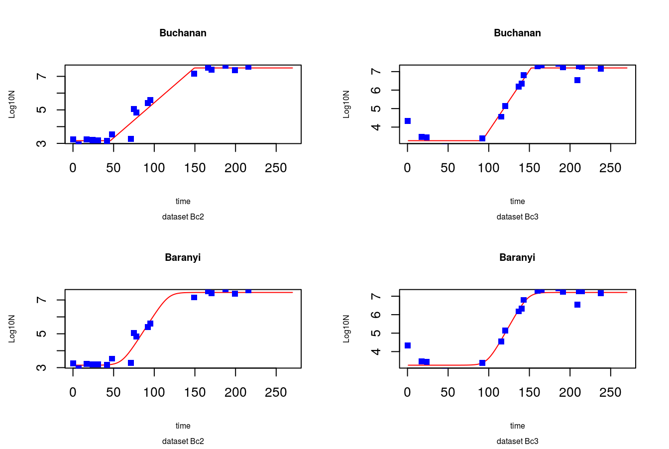
Figure 8.6: Predicted values vs. data points
Fit seems to be quite reasonable. Finally lets check the parameters of models:
summary(buch2.nlsLM)$parameters## Estimate Std. Error t value Pr(>|t|)
## lag 46.05276132 6.39164691 7.205148 2.096717e-06
## mumax 0.09676246 0.01095127 8.835730 1.493145e-07
## LOG10N0 3.16285715 0.14910019 21.212965 3.852824e-13
## LOG10Nmax 7.50200000 0.17641773 42.524072 6.902309e-18summary(buch3.nlsLM)$parameters## Estimate Std. Error t value Pr(>|t|)
## lag 91.8457093 5.86309056 15.665067 3.979643e-11
## mumax 0.1501464 0.02126317 7.061337 2.691088e-06
## LOG10N0 3.2650000 0.16502452 19.784939 1.130406e-12
## LOG10Nmax 7.1975000 0.14291542 50.361954 4.696585e-19summary(bar2.nlsLM)$parameters## Estimate Std. Error t value Pr(>|t|)
## lag 60.0785947 5.80981604 10.340877 1.719577e-08
## mumax 0.1727468 0.03662681 4.716403 2.328926e-04
## LOG10N0 3.1450278 0.12117868 25.953641 1.666670e-14
## LOG10Nmax 7.4431721 0.13857817 53.710999 1.686156e-19summary(bar3.nlsLM)$parameters## Estimate Std. Error t value Pr(>|t|)
## lag 98.0820517 7.6186089 12.874011 7.381774e-10
## mumax 0.1808689 0.0392226 4.611345 2.889377e-04
## LOG10N0 3.2651346 0.1592311 20.505639 6.509231e-13
## LOG10Nmax 7.2034057 0.1467807 49.075958 7.086484e-198.4 Going further
Now you have all the necessary techniques, to go beyond the scope of this book. With more data sets you will be easily able to make prediction how \(\mu_{max}\) changes along temperature gradient. From standard error it will be fairly easy to calculate standard deviation, and use it for estimation of your parameters distribution. Than you can use random sampling for stochastic simulations. With some effort and clever queries, you will find how to make beautiful plots using powerful ggplot2 package and its extensions. Of course, in the beginning it will take some time, and probably frustration, but all in all you are now using one of the most powerful and differentiated IT tools. It’s only upon you how you will use the knowledge.
8.5 Copy-paste data set
BcDF <- data.frame(Time = c(0.00, 17.00, 43.00, 66.50, 139.50, 187.00, 283.00,
                            478.00, 526.00, 550.00, 605.50, 887.00,
                            0.00, 7.00, 17.00, 24.00, 25.00, 31.00, 42.00,
                            48.00, 54.00, 71.00, 75.00, 78.00, 92.00, 95.00,
                            149.00, 166.00, 170.50, 187.50, 199.00, 216.00,
                            0.00, 17.62, 23.82, 40.43, 46.18, 71.17, 92.03,
                            115.17, 120.10, 137.05, 140.40, 143.08, 159.85,
                            165.25, 185.68, 191.27, 209.27, 210.95, 214.55,
                            237.90,
                            0.00, 16.22, 19.02, 20.93, 23.40, 40.98, 45.23,
                            47.98, 66.07, 69.35, 71.68, 89.60, 161.32, 166.12,
                            187.20, 190.45, 209.13,
                            0.00, 1.13, 2.05, 2.93, 4.08, 4.98, 6.02, 6.90,
                            8.02, 9.02, 10.08, 10.95, 12.08, 12.98, 14.13,
                            15.38, 16.22, 19.75),
                   LogC = c(3.25, 3.54, 3.53, 3.40, 3.34, 3.38, 3.40, 5.78,
                            7.00, 6.70, 7.34, 6.48, 3.25, 2.95, 3.23, 3.20,
                            3.18, 3.18, 3.15, 3.53, 2.78, 3.28, 5.04, 4.85,
                            5.41, 5.60, 7.15, 7.52, 7.41, 7.63, 7.36, 7.59,
                            4.33, 3.48, 3.45, 2.76, 2.92, 2.65, 3.39, 4.56,
                            5.15, 6.18, 6.34, 6.80, 7.30, 7.35, 7.43, 7.24,
                            6.54, 7.28, 7.27, 7.17, 2.54, 2.30, 2.24, 2.40,
                            2.54, 5.15, 5.73, 6.42, 7.72, 7.94, 7.73, 7.95,
                            8.02, 7.88, 7.99, 7.95, 7.32, 3.67, 3.51, 3.55,
                            3.70, 3.98, 4.46, 4.77, 4.92, 5.28, 6.24, 6.44,
                            6.92, 7.17, 7.18, 7.36, 7.48, 7.68, 7.98),
                   Temp = c(rep(16, times = 12), rep(22, times = 20),
                            rep(15, times = 20), rep(20, times = 17),
                            rep(30, times = 18)),
                   resID = c(rep('Bc1', times = 12), rep('Bc2', times = 20),
                             rep('Bc3', times = 20), rep('Bc4', times = 17),
                             rep('Bc5', times = 18)))